COLD-PlaceScans Dataset
Overview
 |
 |
 |
 |
|---|---|---|---|
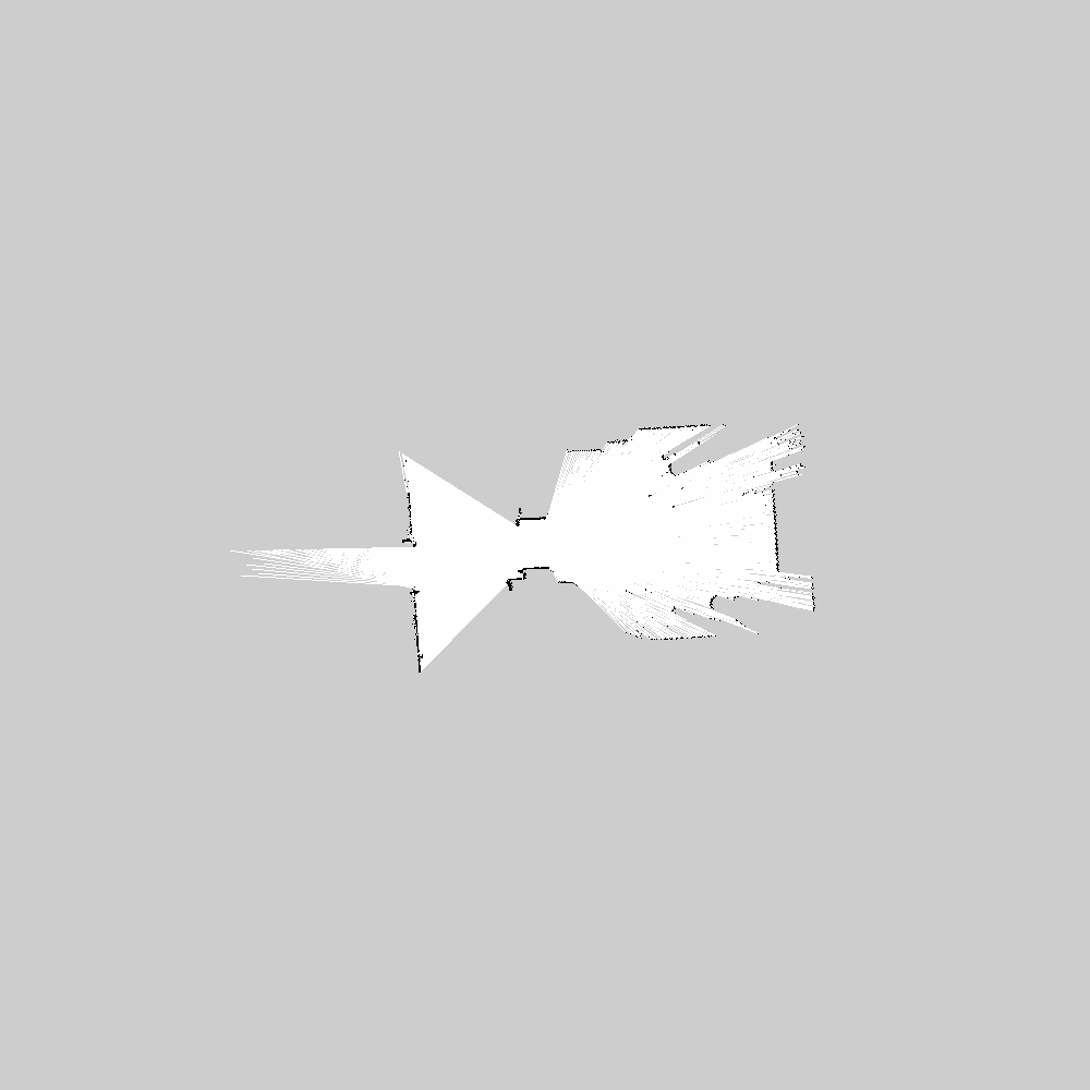
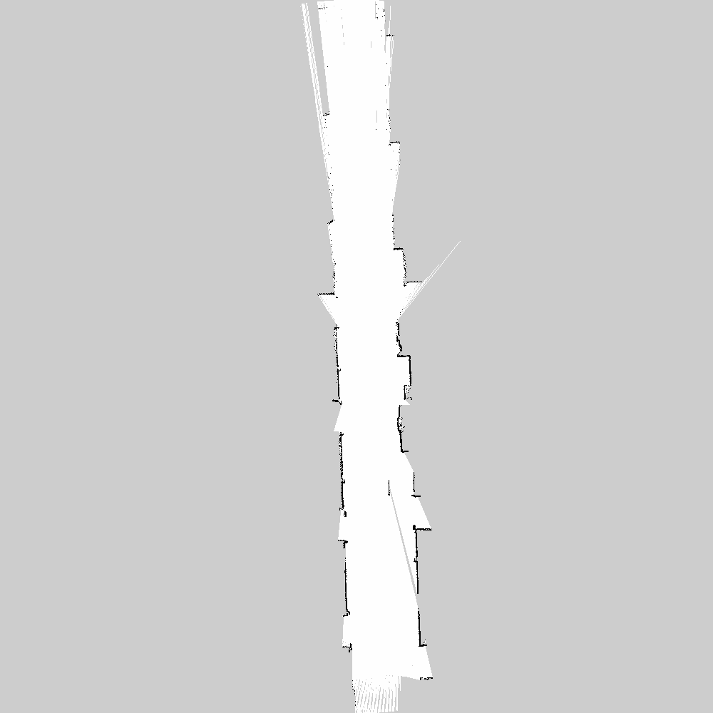
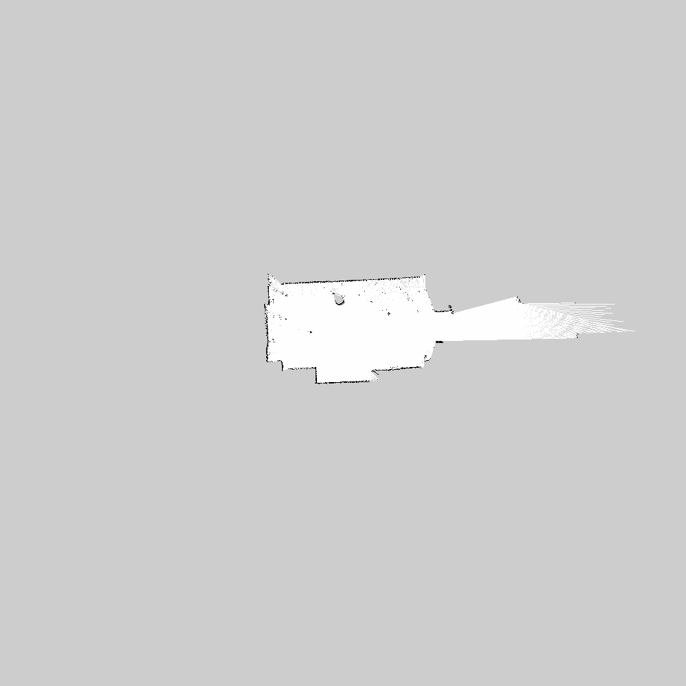
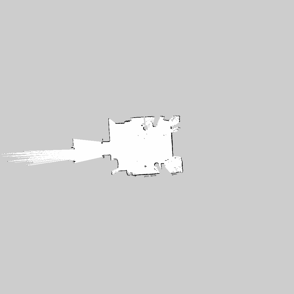
| Doorway | Corridor | One-person office | Two-person office |
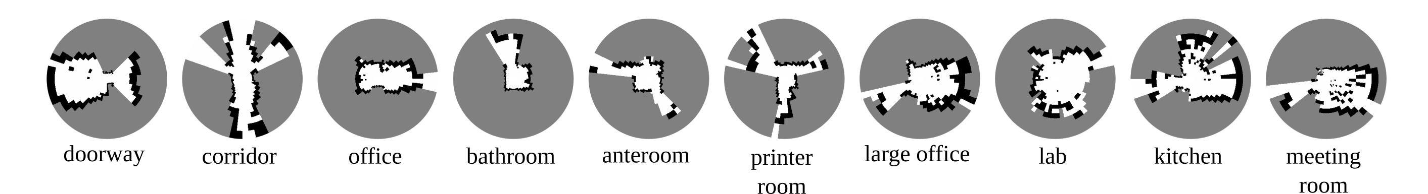
The COLD-PlaceScans Dataset was primarily collected to develop a unified model of geometry and semantics of a robot's local environments. As such, it contains rangefinder-based geometric representation of local environments, named place scan, with their semantic labels. The place scan is a novel robotcentric representation of a local environment such that a robot can accumulate the knowledge about its surroundings and virtually see 360-degree around. Such representation was motivated by the current success of deep learning methods in image recognition tasks.
Details
Format
Place scans are stored in place_scans directory for each sequence. Their file names are in the format of {PLACE_SCAN_COUNT}_{TIMESTAMP}_{ROOM_ID}.png, where ROOM_ID further consists of {FLOOR_LEVEL}-{ROOM_CATEGORY}-{CATEGORY_INSTANCE_ID}.
For example, cold-stockholm/floor4_cloudy_a1/00513_t1205846015.111_l4-2PO-1.png encodes the following information.
- The place scan was taken in a building in Stockholm
- The place scan is 513th in the
floor4_cloudy_a1sequence. - The timestamp in Unix epoch time is 1205846015.111.
- The room is the 1st instance of two-person office in the 4th floor.
The below is all the ROOM_CATEGORY labels in our dataset and their meaning:
| Stockholm | Freiburg | Saarbrücken | Label | Room category | |
|---|---|---|---|---|---|
| 1PO | 1PO | 1PO | 1PO | One-person office | |
| 2PO | 2PO | 2PO | 2PO | Two-person office | |
| AT | BA | BA | AT | Anteroom | |
| BA | CR | CF | BA | Bathroom | |
| CR | DW | CR | CF | Conference room | |
| DW | KT | DW | CR | Corridor | |
| EV | LO | PT/PA | DW | Doorway | |
| KT | PT | RL | EV | Elevator | |
| LMR | ST | TR | KT | Kitchen | |
| LR | LMR | Large meeting room | |||
| MPO | LO | Large office | |||
| MR | LR | Living room | |||
| PRO | MPO | Multi-person office | |||
| PT | MR | Meeting room | |||
| RL | PRO | Professor's office | |||
| WS | PT/PA | Printer area | |||
| RL | Robot lab | ||||
| ST | Stairs | ||||
| TR | Terminal Room | ||||
| WS | Workshop |
Each sequence of place scans are accompanied with place_scans.dat file. This file contains the result of raytracing on the place scans. Each line corresponds to a place scan and has the following format.
{ID} {TIMESTAMP} {#RAYS} {READINGS}... {MIN_ANGLE} {ANGLE_INCREMENT} {MAX_RANGE} {MIN_RANGE}
We generated this file with a setting such that #RAYS=7200, MIN_ANGLE=-Pi, ANGLE_INCREMENT=2Pi/#RAYS, MAX_RANGE=10, MIN_RANGE=0.
Acquisition Procedure
Place scans were generated while a robot was exploring a new environment.
- Integrate incoming laser scans to generate an occupancy grid map.
- Filter noise such as small blobs in empty space and holes on walls.
- Raytrace from the robot’s estimated location in the grid map until rays hit either an unknown or occupied cell.
- Search around the hit occupied cells and recover the occupied vicinity that were occuluded in the last step.
- Raytrace back from each of the recovered cells to the robot's location.
- Save the cells of the original grid map which were raytraced or raytraced back.
In detail, the first step used the GMapping [1] implementation of the Rao-Blackwellized particle filters. The second filtering step was done to smooth the following raytracing. We removed the small blobs by closing, meaning dilation followed by erosion and interpolated holes by opening, the opposite transformation of closing [2]. The strength of the filter was handtuned so that it removes small obstacles like legs of a table but retains major structures. By raytracing in the third step, we can basically extract a part of the grid map which represents the room where the robot is located because all the other parts is occuluded by the wall.
However, we continue to the following step 4 and step 5 to retain the corner structures of objects, which we cannot capture by naive raytracing. The range of recovery in the fourth step is also a parameter. We set the value low to minimize external influences such as raytracing back from the outer corridors. It happens because we search the vicinity cells by BFS, and the occupied cells of corridor are often connected to the occupied cells of the walls because of the structure.
Annotations
The place scans were annotated with the semantic category of the place. This can be done if
- the map of the building with room category annotation
- the robot's location in the map when the place scan was taken
are available. Given these, you can look up the robot's location in the annotated map and label the place scan accordingly.
We created the "canonical" occupancy grid map by GMapping and annotated them by hand. Then, we localized our robot on the canonical map from sensor readings by Adaptive Monte Carlo localization (AMCL) while place scan acquisition. The place scans were taken at 4Hz and the poses were estimated at TODO XHz, so by matching closest timestamps, we can estimate the canonical robot's pose when the place scan was taken. Some error can be induced because of the AMCL's probabilistic nature and the timestamp difference between place scan and pose, but we didn't find any errorneous labeling after through eye scanning.
Download
Please download the following repositories, one for each building:
then, from the directory of each repository, run
$ bash download_place_scans.sh
(or mark the download_place_scans.sh as executable then execute it) The files should be downloaded to a place_scans directory, created in the repository directory.
Generate Polar Scans
We provide some code to convert a cartesian space place scan to a polar space place scan (abbrv. polar scan) like above (56 by 21):
import matplotlib.pyplot as plt
import matplotlib as mpl
import numpy as np

#56x21
class common:
    resolution      = 0.02
    num_angle_cells = 56
    min_radius      = 0.3
    max_radius      = 5
    radius_factor   = 1.15

    angles = np.linspace(-180, 180, num_angle_cells+1)
    r=min_radius
    radiuses=[r]
    v = 0.04
    while r<max_radius:
        r = r+v
        radiuses.append(r)
        v*=radius_factor
    radiuses = np.array(radiuses)
    num_radius_cells = len(radiuses)-1

def pixel_to_polar(scan_size, x, y):
    """Convert pixel coordinate to polar cell coordinate."""
    c_x = scan_size[0]//2
    c_y = scan_size[1]//2
    x = x - c_x
    y = y - c_y
    r = np.sqrt(x**2 + y**2) * common.resolution
    alpha = np.arctan2(-y, x) # angles go clockwise with the
    return (r, np.degrees(alpha))

def scan_to_polar(scan_image):
    ys,xs = np.meshgrid(np.arange(scan_image.shape[0])+0.5,
                        np.arange(scan_image.shape[1])+0.5)
    rr, aa = pixel_to_polar(scan_image.shape, xs, ys)
    aa = np.digitize(aa, common.angles) - 1
    # Additional cell for stuff near the robot
    rr = np.digitize(rr, np.r_[0, common.radiuses]) - 1
    polar_scan_elems = [[[] for _ in range(common.num_angle_cells)]
                        for _ in range(common.num_radius_cells)]
    for x in range(scan_image.shape[0]):
        for y in range(scan_image.shape[1]):
            r = rr[x,y]
            a = aa[x,y]
            if r>0 and r<=common.num_radius_cells:
                polar_scan_elems[r-1][a].append(scan_image[x,y])
    for r in range(common.num_radius_cells):
        for a in range(common.num_angle_cells):
            vals=polar_scan_elems[r][a]
            free_count = sum(1 for i in vals if i>250)
            occupied_count = sum(1 for i in vals if i<10)
            unknown_count = len(vals) - free_count - occupied_count
            if not vals: # No elements!
            raise Exception("No elements in %s %s" % (r, a))
            if occupied_count/len(vals) > 0.01:
                    val = 1
            elif free_count/len(vals) > 0.01:
                    val = 0
            else:
                val = -1
            polar_scan_elems[r][a]=val
    return np.array(polar_scan_elems)

def plot_polar_scan(polar_scan, save_img_path):
    polar_scan = polar_scan.reshape(common.num_radius_cells, common.num_angle_cells)
    a, r = np.meshgrid(np.radians(common.angles), common.radiuses)
    ax = plt.subplot(111, projection='polar')
    ax.set_theta_zero_location("S")
    ax.set_theta_direction(-1)
    ax.set_yticklabels([])
    ax.set_xticklabels([])
    ax.spines['polar'].set_visible(False)
    cmap = mpl.colors.LinearSegmentedColormap.from_list('mycmap', [(0, 'gray'),
                                                        (0.5, 'white'),
                                                        (1, 'black')])

    ax.pcolormesh(a, r, polar_scan+1, cmap=cmap, edgecolors="none")
    plt.savefig(save_img_path, transparent=True)
    plt.clf()
Citation
The paper for COLD database will be available soon.
Reference
[1] https://openslam-org.github.io/gmapping.html
[2] https://docs.opencv.org/3.0-beta/doc/py_tutorials/py_imgproc/py_morphological_ops/py_morphological_ops.html